|
General Description : The geometric system
correction is the rotation and the coordinate transformation of the
line of sight vectors of detectors to the earth Greenwich coordinate
system using only the engineering information from the instrument and
the spacecraft to identify the observed points by the detectors. The
observed point on the surface is identified by the intersection of
the earths surface and an extended line-of-sight vector The
engineering information from the instrument and the spacecraft are
called the supplementary data and the ancillary data, respectively.
The geometric system correction is almost the same for the three
subsystems, except for selected numbers of vectors to be transformed.
Figure 2-6 shows the geometric system correction flow.
The image data are divided into blocks for both of the cross-track
and the along-track directions. The block sizes are as follows.
VNIR bands 1, 2, 3N: 410 x 400 pixels
VNIR band 3B: 500 x 400 pixels
SWIR all bands: 20 x 20 pixels
TIR all bands: 72 x 70 pixels
These values were decided by considering the distortion of optical
images on the focal plane in the cross-track direction and spacecraft
stability in the along-track direction. The coordinate
transformations are carried out only for the line-of-sight vectors of
selected detectors. The numbers of the selected detectors are 11, 104
and 11 for VNIR, SWIR and TIR bands, respectively, which correspond
to the number of the corner for each block of Level-0 images in the
cross-track direction. Dummy detectors will have to be introduced to
compensate for and then to completely define the block at the end of
the cross-track direction.
The geometric system correction is divided into several parts as
follows:
- The pointing correction
- The coordinates transformation from Navigation Base Reference
of the spacecraft to the Orbital Reference Frame
- The coordinates transformation from the Orbital Reference
Coordinate Frame to the Earth Inertial coordinate Frame
- The coordinates transformation from the Earth Inertial
Coordinate Frame to the Earth Greenwich Coordinate Frame
- Identification of the intersection of the Earth surface and an extention of
the line of sight vector
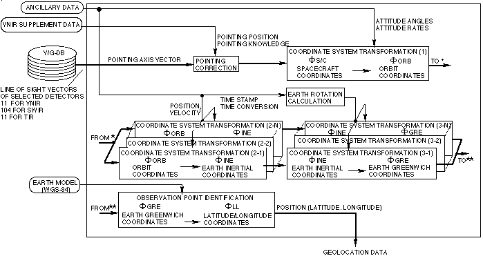
Figure 2-6 Geometric system correction flow
Pointing Correction : The line of sight
vectors in the geometric data base are those for the reference
pointing angles (nominal nadir direction). The line of sight vectors
are changed using the pointing position and knowledge from the
supplementary data. The pointing axes information in the geometric
data base are used for the transformation of the line-of-sight
vectors due to change in the pointing position.
The line of sight vector changes with the rotation for the
pointing axis by an angle of β from S0 to S as
follows.
|
|
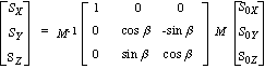
|
(2-1)
|
where
S0x, S0y, S0z : x, y , z
components of the line of sight vector S0 before
pointing,
Sx, Sy, Sz : x, y, x
components of the line of sight vector S after pointing,
Px, Py, Pz : x, y, z componets of
the pointing axes unit vector in the NBR Coordinate Frame.
Figure 2-7 shows the relation between the pointing axis and the
NBR Coordinate Frame. The angles Dqyaw
and Dq
pitch are the yaw and the pitch rotation
angles, respectively, to coalign the XNBR to the pointing
axis.
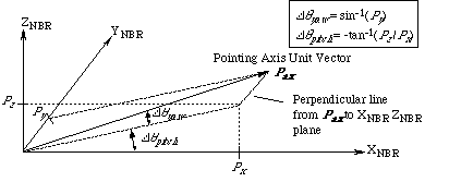
Figure 2-7 Pointing Axis Vector in NBR Coordinate Frame
Spacecraft-to-Orbit Coordinates : The
spacecraft coordinates are slightly different from the orbit
coordinates. The difference originates from the spacecraft attitude
control accuracy and is provided as the attitude angle data in the
spacecraft ancillary information. The orbit coordinate system is
right-handed and orthogonal. The +z-axis is a line from the
spacecraft center of mass to the center of the earth. The +y-axis is
a line normal to the z-axis and the spacecraft instantaneous velocity
vector (negative orbit normal direction). The x-axis completes the
right hand set. This process is carried out by using attitude angles
and rates in the ancillary data.
The line of sight vectors in the Spacecraft NBR Coordinate Frame
can be converted to the expression in the Orbital Reference Frame
using the attitude angle data in the spacecraft ancillary data as
follows.
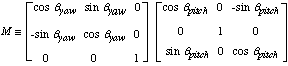
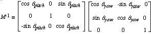
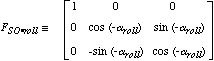
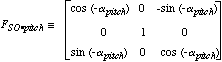
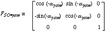
|
|
SOR = FSO•yaw
FSO•pitch FSO•roll S
|
(2-6)
|
where S : the line of sight vector expressed in the NBR Coordinate
Frame,
SOR : the line of sight vector expressed in the Orbit
Reference Coordinate Frame,
aroll, a
pitch , a
yaw : roll, pitch, yaw components of the
attitude data, respectively, in the spacecraft ancillary data
Orbit-to-Earth Inertial Coordinates : This
process is the coordinate transformation to earth-centered
coordinates in inertial space. Two-dimensional array vectors can be
obtained by this transformation using the spacecraft movement. The
array dimension for one observation depends on each observation
period, that is, number of pixels in the along-track direction. This
process is carried out by using position and velocity information in
the ancillary data. The Precession and the Nutation effects are
considered to be the more accurate geolocation data, since the
spacecraft position information is based on the mean of the J2000.0
coordinate frame, which is the earth inertial coordinates at noon of
January 1st, 2000.
The line of sight vectors in the Orbital Reference Coordinate
Frame can be converted to the expression in the Earth Inertial
Coordinate Frame as follows.
|
|
SEI = FOI SOR
|
(2-10)
|
|
where
|
SOR : the line of sight vector expressed in
the Orbit Reference Coordinate Frame,
SEI : the line of sight vector expressed in the
Eartt Inertial Coordinate Frame,
|
|
|
FOI = (Tx
Ty Tz )
|
(2-11)
|
Tx Ty Tz : unit vector components of x, y and z
axes of the Orbital Coordinate Frame expressed in the
Earth Inertial Coordinate Frame and defined as
|
|
|
Tx = Ty x
Tz
Ty = unit (-R x V )
Tz = unit (-R )
|
(2-12)
|
R ,V : the spacecraft position and velocity
vectors expressed in the Earth Inertial Frame
|
For more accurate calculation the Precession matrix P and the
Nutation matrix N shall be applied to the line of sight vector
SEI in the Earth Inertial Coordinate Frame.
Earth Inertial-to-Earth Fixed coordinates :
This process is the coordinate transformation to the earth centered
and earth-fixed coordinates, and carried out by using the earth
rotation values calculated from the time information in the ancillary
data. The UTC time, which is provided from the spacecraft, is
converted to the UT1 to calculate the exact earth rotation angle.
The line of sight vectors in the Earth Inertial Coordinate Frame
can be converted to the expression in the Earth Fixed Coordinate
Frame as follows.
|
|
SEF= FIF SEI
|
(2-13)
|
|
where
|
SEI : the line of sight vector expressed in
the Eartt Inertial Coordinate Frame,
SEF : the line of sight vector expressed in the
Eartt Fixed Coordinate Frame,
|
|
|
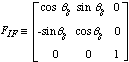
|
(2-14)
|
|
|
qg : Greenwich true
sidereal hour angle.
|
Eath Surface Identification : The observation
point is identified from the intersection of the earth surface and an
extension of the line-of-sight vector. The WGS-84 is used as the
earth surface model.
The observing earth surface can be identified calculating the
crossing point between the extension line of the LOS vector and the
earth surface. The extension line of the LOS vector can be expressed
as follows.
|
|
x = X + SEF•x r
y = Y + SEF•y r
z = Z + SEF•z r
|
(2-15)
|
|
where
|
SEF•x , SEF•y ,
SEF•z : x, y, z components of the LOS vector
SEF in the Earth Fixed Coordinate Frame,
X, Y, Z : x, y, z components of the Spacecraft position
vector in the Earth Fixed Coordinate Frame
r : parameter.
|
The earth surface can be expressed as follows.
|
|
(x 2 + y
2)/a 2 + z 2/b
2 = 1
|
(2-16)
|
|
where
|
a = 6378136m (Earth radius at equator--WGS-84),
b = a (1 - f ) (Earth radius at pole----WGS-84),
f = 1/298.2572 .
|
(2-17)
|
The intersection can be calculated from eqs.(2-15) and (2-16). When
the observing point is expressed as Px, Py, and Pz , the geocentric
latitude y and the longitude l
can be expressed as follows.
|
|
y =
tan-1{Pz
/(Px2 +
Py2)1/2}
|
(2-18)
|
|
|
l =
tan-1(Py /Px )
|
(2-19)
|
System Correction Accuracy : Table 2-2 shows
the pixel geolocation knowledge as a result of the geometric system
correction considering both the spacecraft and the instrument
contributions. Total ASTER pixel geolocation knowledge is decided by
the spacecraft position knowledge, the spacecraft pointing knowledge
and ASTER pointing knowledge. Only the pixel geolocation knowledge
of VNIR is considered, since the SWIR and TIR bands will be
coregistered to VNIR band 2 as a reference band in the Level-1
processing .
Table 2-2 Pixel Geolocation Knowledge
|
|
Specification
|
Dynamic Error (3s)
|
Static Error (3s)
|
|
Along-track (m)
|
Spacecraft*1
|
±
342
|
±
28
|
±
111
|
|
ASTER/VNIR
|
±
205
|
±
38
|
±
99
|
|
Total
|
± 431
*2
|
±
47
|
±
149
|
|
Cross-track (m)
|
Spacecraft*1
|
±
342
|
±
25
|
±
148
|
|
ASTER/VNIR
|
±
205
|
±
48
|
±
103
|
|
Total
|
± 437
*2
|
±
54
|
±
180
|
*1: Three non-optimal 9 minute TDRS contacts per orbit, GJM2
Geopotential ( 30 x 30), solar flux of 175, 5 % Cd error, TDRS
ephemeris error of 75 meters. Two star trackers, rigid body/low frequency pointing knowledge error removed.
*2: Slightly larger than RSS of two values (Spacecraft and ASTER instrument), because of unallocated margin.
|